How to Upload Text File and Display It in Shiny
Building a Shiny app to upload and visualize spatio-temporal data
In this chapter we bear witness how to build a Shiny web application to upload and visualize spatio-temporal data (Chang et al. 2021). The app allows to upload a shapefile with a map of a region, and a CSV file with the number of illness cases and population in each of the areas in which the region is divided. The app includes a variety of elements for interactive information visualization such as a map congenital with leaflet (Cheng, Karambelkar, and Xie 2021), a table built with DT (Xie, Cheng, and Tan 2021), and a time plot congenital with dygraphs (Vanderkam et al. 2018). The app as well allows interactivity by giving the user the possibility to select specific data to exist shown. To build the app, nosotros apply data of the number of lung cancer cases and population in the 88 counties of Ohio, United states of america, from 1968 to 1988 (Effigy 15.1).
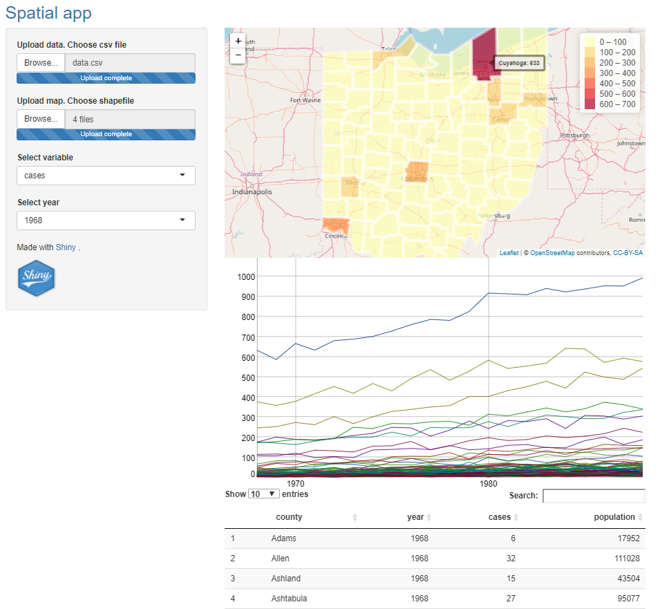
Effigy 15.1: Snapshot of the Shiny app to upload and visualize spatio-temporal data.
Shiny
Shiny is a spider web application framework for R that enables to build interactive spider web applications. Chapter 13 provides an introduction to Shiny and examples, and here nosotros review its basic components. A Shiny app can exist built past creating a directory (called, for example, appdir) that contains an R file (chosen, for instance, app.R) with three components:
- a user interface object (
ui) which controls the layout and appearance of the app, - a
server()function with the instructions to build the objects displayed in theui, and - a phone call to
shinyApp()that creates the app from theui/serverpair.
Shiny apps contain input and output objects. Inputs permit users interact with the app by modifying their values. Outputs are objects that are shown in the app. Outputs are reactive if they are built using input values. The following code shows the content of a generic app.R file.
# load the shiny package library(shiny) # define user interface object ui <- fluidPage( * Input(inputId = myinput, label = mylabel, ...) * Output(outputId = myoutput, ...) ) # ascertain server() function server <- function(input, output){ output$myoutput <- render*({ # code to build the output. # If it uses an input value (input$myinput), # the output volition exist rebuilt whenever # the input value changes })} # telephone call to shinyApp() which returns the Shiny app shinyApp(ui = ui, server = server) The app.R file is saved inside a directory chosen, for instance, appdir. And then, the app tin can be launched by typing runApp("appdir_path") where appdir_path is the path of the directory that contains app.R, or past clicking the Run button of RStudio.
Setup
To build the Shiny app of this example, we need to download the folder appdir from the volume webpage and save information technology in our computer. This folder contains the following subfolders:
-
informationwhich contains a file calleddata.csvwith the data of lung cancer in Ohio, and a folder calledfe_2007_39_countywith the shapefile of Ohio, and -
wwwwith an image of a Shiny logo calledimageShiny.png.
Structure of app.R
We start creating the Shiny app past writing a file called app.R with the minimum lawmaking needed to create a Shiny app:
We relieve this file with the proper noun app.R inside a directory chosen appdir. Then, we tin launch the app by clicking the Run App button at the tiptop of the RStudio editor or by executing runApp("appdir_path") where appdir_path is the path of the directory that contains the app.R file. The Shiny app created has a bare user interface. In the post-obit sections, nosotros include the elements and functionality we wish to have in the Shiny app.
Layout
We build a user interface with a sidebar layout. This layout includes a championship panel, a sidebar panel for inputs on the left, and a primary panel for outputs on the right. The elements of the user interface are placed inside the fluidPage() office and this permits the app to adjust automatically to the dimensions of the browser window. The title of the app is added with titlePanel(). And so we write sidebarLayout() to create a sidebar layout with input and output definitions. sidebarLayout() takes the arguments sidebarPanel() and mainPanel(). sidebarPanel() creates a a sidebar panel for inputs on the left. mainPanel() creates a main panel for displaying outputs on the right.
We can add together content to the app by passing it as an argument to titlePanel(), sidebarPanel(), and mainPanel(). Here we take added texts with the description of the panels. Annotation that to include multiple elements in the same panel, nosotros need to split up them with commas.
HTML content
Here nosotros add a title, an image and a website link to the app. First nosotros add the championship "Spatial app" to titlePanel(). We want to show this title in blueish so nosotros use p() to create a paragraph with text and gear up the style to the #3474A7 color.
titlePanel(p("Spatial app", fashion = "colour:#3474A7")), And then we add together an image with the img() role. The images that we wish to include in the app must exist in a folder named www in the same directory equally the app.R file. Nosotros employ the image called imageShiny.png and put it in the sidebarPanel() past using the following instruction.
sidebarPanel(img(src = "imageShiny.png", width = "70px", height = "70px")), Hither src denotes the source of the prototype, and top and width are the image pinnacle and width in pixels, respectively. Nosotros also add together text with a link referencing the Shiny website.
p("Fabricated with", a("Shiny", href = "http://shiny.rstudio.com"), "."), Note that in sidebarPanel() we need to write the office to generate the website link and the role to include the prototype separated with a comma.
sidebarPanel( p("Fabricated with", a("Shiny", href = "http://shiny.rstudio.com"), "."), img(src = "imageShiny.png", width = "70px", pinnacle = "70px")), Below is the content of app.R we take until at present. A snapshot of the Shiny app is shown in Figure 15.2.
library ( shiny ) # ui object ui <- fluidPage ( titlePanel ( p ( "Spatial app", style = "color:#3474A7" ) ), sidebarLayout ( sidebarPanel ( p ( "Made with", a ( "Shiny", href = "http://shiny.rstudio.com" ), "." ), img ( src = "imageShiny.png", width = "70px", tiptop = "70px" ) ), mainPanel ( "master panel for outputs" ) ) ) # server() server <- function ( input, output ) { } # shinyApp() shinyApp (ui = ui, server = server ) 
FIGURE 15.2: Snapshot of the Shiny app after including a title, an image and a website link.
Read data
Now we import the information nosotros want to show in the app. The data is in the folder called data in the appdir directory. To read the CSV file data.csv, we employ the read.csv() function, and to read the shapefile of Ohio that is in the folder fe_2007_39_county, nosotros use the readOGR() function of the rgdal package.
We but demand to read the information once then we write this code at the showtime of app.R exterior the server() function. By doing this, the code is not unnecessarily run more once and the performance of the app is not decreased.
Calculation outputs
Now we show the data in the Shiny app by including several outputs for interactive visualization. Specifically, we include HTML widgets created with JavaScript libraries and embedded in Shiny by using the htmlwidgets package (Vaidyanathan et al. 2021). The outputs are created using the following packages:
- DT to display the data in an interactive table,
- dygraphs to display a fourth dimension plot with the data, and
- leaflet to create an interactive map.
Outputs are added in the app past including in ui an *Output() function for the output, and adding in server() a render*() function to the output that specifies how to build the output. For example, to add a plot, we write in the ui plotOutput() and in server() renderPlot().
Table using DT
We show the data in data with an interactive tabular array using the DT packet. In ui we use DTOutput(), and in server() we utilise renderDT().
Time plot using dygraphs
We bear witness a fourth dimension plot with the data with the dygraphs package. In ui we use dygraphOutput(), and in server() we use renderDygraph(). dygraphs plots an extensible fourth dimension serial object xts. We can create this type of object using the xts() role of the xts packet (Ryan and Ulrich 2020) specifying the values and the dates. The dates in data are the years of column yr. For now we cull to plot the values of the variable cases of information.
Nosotros need to construct a xts object for each canton and then put them together in an object called dataxts. For each of the counties, we filter the information of the county and assign it to datacounty. So we construct a xts object with values datacounty$cases and dates as.Appointment(paste0(data$yr, "-01-01")). Then we assign the name of the counties to each xts (colnames(dataxts) <- counties) so county names tin exist shown in the legend.
dataxts <- NULL counties <- unique ( data $ county ) for ( l in ane : length ( counties ) ) { datacounty <- information [ data $ county == counties [ l ], ] dd <- xts ( datacounty [, "cases" ], every bit.Date ( paste0 ( datacounty $ year, "-01-01" ) ) ) dataxts <- cbind ( dataxts, dd ) } colnames ( dataxts ) <- counties Finally, we plot dataxts with dygraph(), and utilise dyHighlight() to allow mouse-over highlighting.
dygraph ( dataxts ) %>% dyHighlight (highlightSeriesBackgroundAlpha = 0.2 ) We customize the legend then that only the proper noun of the highlighted serial is shown. To do this, one option is to write a css file with the instructions and pass the css file to the dyCSS() role. Alternatively, we can set the css directly in the code as follows:
dygraph ( dataxts ) %>% dyHighlight (highlightSeriesBackgroundAlpha = 0.two ) -> d1 d1 $ ten $ css <- " .dygraph-legend > bridge {display:none;} .dygraph-legend > span.highlight { brandish: inline; } " d1 The complete code to build the dygraphs object is the post-obit:
library ( dygraphs ) library ( xts ) # in ui dygraphOutput (outputId = "timetrend" ) # in server() output $ timetrend <- renderDygraph ( { dataxts <- NULL counties <- unique ( data $ county ) for ( fifty in i : length ( counties ) ) { datacounty <- data [ information $ county == counties [ l ], ] dd <- xts ( datacounty [, "cases" ], as.Engagement ( paste0 ( datacounty $ yr, "-01-01" ) ) ) dataxts <- cbind ( dataxts, dd ) } colnames ( dataxts ) <- counties dygraph ( dataxts ) %>% dyHighlight (highlightSeriesBackgroundAlpha = 0.2 ) -> d1 d1 $ x $ css <- " .dygraph-fable > bridge {display:none;} .dygraph-legend > span.highlight { display: inline; } " d1 } ) Map using leaflet
Nosotros use the leaflet packet to build an interactive map. In ui we use leafletOutput(), and in server() we use renderLeaflet(). Inside renderLeaflet() we write the instructions to return a leaflet map. Get-go, we need to add the data to the shapefile and so the values tin be plotted in a map. For at present nosotros choose to plot the values of the variable in 1980. We create a dataset chosen datafiltered with the data respective to that year. Then we add datafiltered to map@data in an order such that the counties in the data lucifer the counties in the map.
datafiltered <- data [ which ( data $ yr == 1980 ), ] # this returns positions of map@information$Proper name in datafiltered$canton ordercounties <- match ( map @ information $ NAME, datafiltered $ county ) map @ data <- datafiltered [ ordercounties, ] Nosotros create the leaflet map with the leaflet() role, create a color palette with colorBin(), and add a legend with addLegend(). For now we choose to plot the values of variable cases. Nosotros as well add together labels with the surface area names and values that are displayed when the mouse is over the map.
library ( leaflet ) # in ui leafletOutput (outputId = "map" ) # in server() output $ map <- renderLeaflet ( { # add data to map datafiltered <- data [ which ( information $ yr == 1980 ), ] ordercounties <- match ( map @ information $ Proper noun, datafiltered $ county ) map @ data <- datafiltered [ ordercounties, ] # create leaflet pal <- colorBin ( "YlOrRd", domain = map $ cases, bins = 7 ) labels <- sprintf ( "%south: %g", map $ county, map $ cases ) %>% lapply ( htmltools :: HTML ) l <- leaflet ( map ) %>% addTiles ( ) %>% addPolygons ( fillColor = ~ pal ( cases ), color = "white", dashArray = "3", fillOpacity = 0.seven, characterization = labels ) %>% leaflet :: addLegend ( pal = pal, values = ~ cases, opacity = 0.7, title = Zip ) } ) Below is the content of app.R we take until now. A snapshot of the Shiny app is shown in Figure 15.3.
library ( shiny ) library ( rgdal ) library ( DT ) library ( dygraphs ) library ( xts ) library ( leaflet ) information <- read.csv ( "data/data.csv" ) map <- readOGR ( "data/fe_2007_39_county/fe_2007_39_county.shp" ) # ui object ui <- fluidPage ( titlePanel ( p ( "Spatial app", style = "color:#3474A7" ) ), sidebarLayout ( sidebarPanel ( p ( "Fabricated with", a ( "Shiny", href = "http://shiny.rstudio.com" ), "." ), img ( src = "imageShiny.png", width = "70px", peak = "70px" ) ), mainPanel ( leafletOutput (outputId = "map" ), dygraphOutput (outputId = "timetrend" ), DTOutput (outputId = "tabular array" ) ) ) ) # server() server <- part ( input, output ) { output $ table <- renderDT ( data ) output $ timetrend <- renderDygraph ( { dataxts <- Zero counties <- unique ( data $ county ) for ( l in ane : length ( counties ) ) { datacounty <- information [ data $ county == counties [ fifty ], ] dd <- xts ( datacounty [, "cases" ], as.Appointment ( paste0 ( datacounty $ twelvemonth, "-01-01" ) ) ) dataxts <- cbind ( dataxts, dd ) } colnames ( dataxts ) <- counties dygraph ( dataxts ) %>% dyHighlight (highlightSeriesBackgroundAlpha = 0.ii ) -> d1 d1 $ x $ css <- " .dygraph-fable > bridge {display:none;} .dygraph-legend > bridge.highlight { display: inline; } " d1 } ) output $ map <- renderLeaflet ( { # Add data to map datafiltered <- data [ which ( information $ year == 1980 ), ] ordercounties <- lucifer ( map @ data $ Proper name, datafiltered $ county ) map @ data <- datafiltered [ ordercounties, ] # Create leaflet pal <- colorBin ( "YlOrRd", domain = map $ cases, bins = seven ) labels <- sprintf ( "%s: %g", map $ county, map $ cases ) %>% lapply ( htmltools :: HTML ) 50 <- leaflet ( map ) %>% addTiles ( ) %>% addPolygons ( fillColor = ~ pal ( cases ), color = "white", dashArray = "3", fillOpacity = 0.seven, characterization = labels ) %>% leaflet :: addLegend ( pal = pal, values = ~ cases, opacity = 0.7, championship = Zip ) } ) } # shinyApp() shinyApp (ui = ui, server = server ) 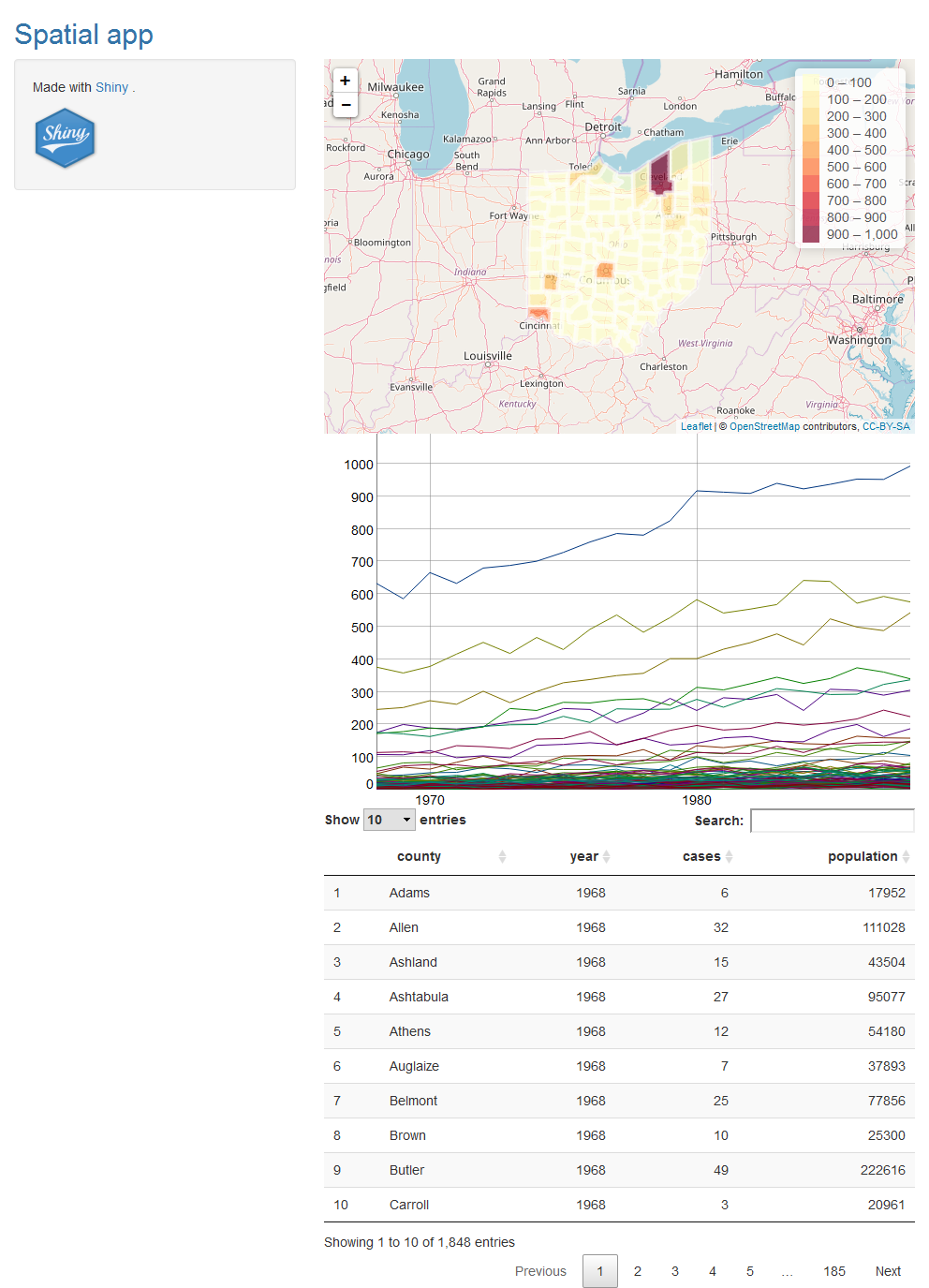
Effigy 15.iii: Snapshot of the Shiny app after including the map, the time plot, and the tabular array.
Adding reactivity
Now we add functionality that enables the user to select a specific variable and year to exist shown. To be able to select a variable, we include an input of a carte containing all the possible variables. And so, when the user selects a particular variable, the map and the time plot will exist rebuilt. To add an input in a Shiny app, we need to identify an input function *Input() in the ui object. Each input function requires several arguments. The get-go ii are inputId, an id necessary to admission the input value, and label which is the text that appears next to the input in the app. We create the input with the menu that contains the possible choices for the variable as follows.
# in ui selectInput ( inputId = "variableselected", label = "Select variable", choices = c ( "cases", "population" ) ) In this input, the id is variableselected, characterization is "Select variable" and choices contains the variables "cases" and "population". The value of this input tin can be accessed with input$variableselected. We create reactivity by including the value of the input (input$variableselected) in the render*() expressions in server() that build the outputs. Thus, when we select a different variable in the menu, all the outputs that depend on the input will be rebuilt using the updated input value.
Similarly, we add a carte du jour with id yearselected and with choices equal to all possible years so nosotros tin select the year nosotros want to come across. When we select a yr, the input value input$yearselected changes and all the outputs that depend on it will be rebuilt using the new input value.
# in ui selectInput ( inputId = "yearselected", label = "Select year", choices = 1968 : 1988 ) Reactivity in dygraphs
In this section we change the dygraphs time plot and the leaflet map then that they are built with the input values input$variableselected and input$yearselected. We change renderDygraph() by writing datacounty[, input$variableselected] instead of datacounty[, "cases"].
# in server() output $ timetrend <- renderDygraph ( { dataxts <- NULL counties <- unique ( data $ county ) for ( l in one : length ( counties ) ) { datacounty <- data [ data $ canton == counties [ 50 ], ] # Change "cases" past input$variableselected dd <- xts ( datacounty [, input $ variableselected ], as.Date ( paste0 ( datacounty $ yr, "-01-01" ) ) ) dataxts <- cbind ( dataxts, dd ) } ... } ) Reactivity in leaflet
We also modify renderLeaflet() past selecting information corresponding to year input$yearselected and plot variable input$variableselected instead of variable cases. We create a new column in map called variableplot with the values of variable input$variableselected and plot the map with the values in variableplot. In leaflet() we change colorBin(), addPolygons(), addLegend() and labels to bear witness variableplot instead of variable cases.
output $ map <- renderLeaflet ( { # Add data to map # Alter 1980 by input$yearselected datafiltered <- information [ which ( information $ yr == input $ yearselected ), ] ordercounties <- match ( map @ data $ NAME, datafiltered $ county ) map @ data <- datafiltered [ ordercounties, ] # Create variableplot # Add this to create variableplot map $ variableplot <- as.numeric ( map @ data [, input $ variableselected ] ) # Create leaflet # CHANGE map$cases by map$variableplot pal <- colorBin ( "YlOrRd", domain = map $ variableplot, bins = seven ) # CHANGE map$cases by map$variableplot labels <- sprintf ( "%s: %grand", map $ canton, map $ variableplot ) %>% lapply ( htmltools :: HTML ) # Alter cases by variableplot l <- leaflet ( map ) %>% addTiles ( ) %>% addPolygons ( fillColor = ~ pal ( variableplot ), color = "white", dashArray = "three", fillOpacity = 0.7, label = labels ) %>% # Change cases past variableplot leaflet :: addLegend ( pal = pal, values = ~ variableplot, opacity = 0.7, title = Cipher ) } ) Note that a better fashion to alter an existing leaflet map is using the leafletProxy() role. Details on how to utilise this office are given in the RStudio website. The content of the app.R file is shown below and a snapshot of the Shiny app is shown in Figure 15.4.
library ( shiny ) library ( rgdal ) library ( DT ) library ( dygraphs ) library ( xts ) library ( leaflet ) information <- read.csv ( "data/information.csv" ) map <- readOGR ( "information/fe_2007_39_county/fe_2007_39_county.shp" ) # ui object ui <- fluidPage ( titlePanel ( p ( "Spatial app", style = "color:#3474A7" ) ), sidebarLayout ( sidebarPanel ( selectInput ( inputId = "variableselected", label = "Select variable", choices = c ( "cases", "population" ) ), selectInput ( inputId = "yearselected", label = "Select year", choices = 1968 : 1988 ), p ( "Fabricated with", a ( "Shiny", href = "http://shiny.rstudio.com" ), "." ), img ( src = "imageShiny.png", width = "70px", tiptop = "70px" ) ), mainPanel ( leafletOutput (outputId = "map" ), dygraphOutput (outputId = "timetrend" ), DTOutput (outputId = "table" ) ) ) ) # server() server <- part ( input, output ) { output $ table <- renderDT ( information ) output $ timetrend <- renderDygraph ( { dataxts <- Naught counties <- unique ( data $ county ) for ( l in one : length ( counties ) ) { datacounty <- data [ data $ county == counties [ l ], ] dd <- xts ( datacounty [, input $ variableselected ], every bit.Date ( paste0 ( datacounty $ year, "-01-01" ) ) ) dataxts <- cbind ( dataxts, dd ) } colnames ( dataxts ) <- counties dygraph ( dataxts ) %>% dyHighlight (highlightSeriesBackgroundAlpha = 0.2 ) -> d1 d1 $ 10 $ css <- " .dygraph-legend > span {brandish:none;} .dygraph-legend > span.highlight { display: inline; } " d1 } ) output $ map <- renderLeaflet ( { # Add data to map # Modify 1980 by input$yearselected datafiltered <- data [ which ( information $ year == input $ yearselected ), ] ordercounties <- lucifer ( map @ data $ NAME, datafiltered $ county ) map @ data <- datafiltered [ ordercounties, ] # Create variableplot # Add together this to create variableplot map $ variableplot <- as.numeric ( map @ data [, input $ variableselected ] ) # Create leaflet # Alter map$cases by map$variableplot pal <- colorBin ( "YlOrRd", domain = map $ variableplot, bins = seven ) # CHANGE map$cases by map$variableplot labels <- sprintf ( "%s: %one thousand", map $ county, map $ variableplot ) %>% lapply ( htmltools :: HTML ) # Change cases by variableplot l <- leaflet ( map ) %>% addTiles ( ) %>% addPolygons ( fillColor = ~ pal ( variableplot ), colour = "white", dashArray = "iii", fillOpacity = 0.7, label = labels ) %>% # Change cases by variableplot leaflet :: addLegend ( pal = pal, values = ~ variableplot, opacity = 0.7, title = Nix ) } ) } # shinyApp() shinyApp (ui = ui, server = server ) 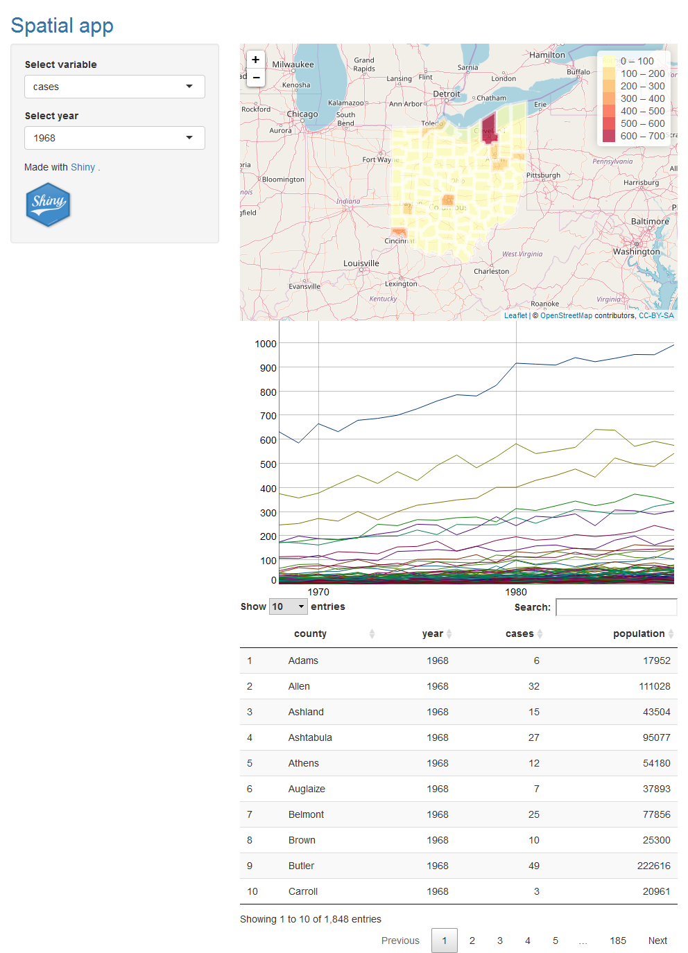
FIGURE xv.4: Snapshot of the Shiny app after calculation reactivity.
Uploading data
Instead of reading the data at the beginning of the app, we may want to permit the user upload his or her own files. In society to do that, we delete the code we previously used to read the data, and add together ii inputs that enable to upload a CSV file and a shapefile.
Inputs in ui to upload a CSV file and a shapefile
Nosotros create inputs to upload the information with the fileInput() role. fileInput() has a parameter called multiple that can exist set to TRUE to permit the user to select multiple files. It also has a parameter called have that can be set to a character vector with the blazon of files the input expects. Here nosotros write two inputs. One of the inputs is to upload the information. This input has id filedata and the input value can be accessed with input$filedata. This input accepts .csv files.
# in ui fileInput(inputId = "filedata", label = "Upload data. Choose csv file", take = c(".csv")), The other input is to upload the shapefile. This input has id filemap and the input value can be accessed with input$filemap. This input accepts multiple files of blazon '.shp', '.dbf', '.sbn', '.sbx', '.shx', and '.prj'.
# in ui fileInput(inputId = "filemap", characterization = "Upload map. Choose shapefile", multiple = TRUE, have = c('.shp','.dbf','.sbn','.sbx','.shx','.prj')), Note that a shapefile consists of dissimilar files with extensions .shp, .dbf, .shx etc. When nosotros are uploading the shapefile in the Shiny app, nosotros demand to upload all these files at once. That is, nosotros need to select all the files and then click upload. Selecting just the file with extension .shp does not upload the shapefile.
Uploading CSV file in server()
We apply the input values to read the CSV file and the shapefile. We do this within a reactive expression. A reactive expression is an R expression that uses an input value and returns a value. To create a reactive expression we use the reactive() office which takes an R expression surrounded by braces ({}). The reactive expression updates whenever the input value changes.
For example, nosotros read the information with read.csv(input$filedata$datapath) where input$filedata$datapath is the data path contained in the value of the input that uploads the information. We put read.csv(input$filedata$datapath) within reactive(). In this way, each time input$filedata$datapath is updated, the reactive expression is reexecuted. The output of the reactive expression is assigned to data. In server(), data can be accessed with data(). information() will exist updated each time the reactive expression that builds is reexecuted.
Uploading shapefile in server()
Nosotros besides write a reactive expression to read the map. We assign the effect of the reactive expression to map. In server(), we access the map with map(). To read the shapefile, we utilise the readOGR() role of the rgdal package. When files are uploaded with fileInput() they accept dissimilar names from the ones in the directory. We first rename files with the actual names and then read the shapefile with readOGR() passing the proper noun of the file with .shp extension.
# in server() map <- reactive ( { # shpdf is a data.frame with the name, size, type and datapath # of the uploaded files shpdf <- input $ filemap # The files are uploaded with names # 0.dbf, one.prj, 2.shp, 3.xml, 4.shx # (path/names are in column datapath) # We demand to rename the files with the actual names: # fe_2007_39_county.dbf, etc. # (these are in column proper noun) # Proper name of the temporary directory where files are uploaded tempdirname <- dirname ( shpdf $ datapath [ 1 ] ) # Rename files for ( i in i : nrow ( shpdf ) ) { file.rename ( shpdf $ datapath [ i ], paste0 ( tempdirname, "/", shpdf $ name [ i ] ) ) } # Now we read the shapefile with readOGR() of rgdal parcel # passing the name of the file with .shp extension. # We employ the function grep() to search the pattern "*.shp$" # within each element of the character vector shpdf$name. # grep(pattern="*.shp$", shpdf$name) # ($ at the stop announce files that finish with .shp, # not only that contain .shp) map <- readOGR ( paste ( tempdirname, shpdf $ proper name [ grep (pattern = "*.shp$", shpdf $ name ) ], sep = "/" ) ) map } ) Handling missing inputs
After calculation the inputs to upload the CSV file and the shapefile, we note that the outputs in the Shiny app render error messages until the files are uploaded (Figure 15.5). Here nosotros change the Shiny app to eliminate these error messages by including code that avoids to show the outputs until the files are uploaded.
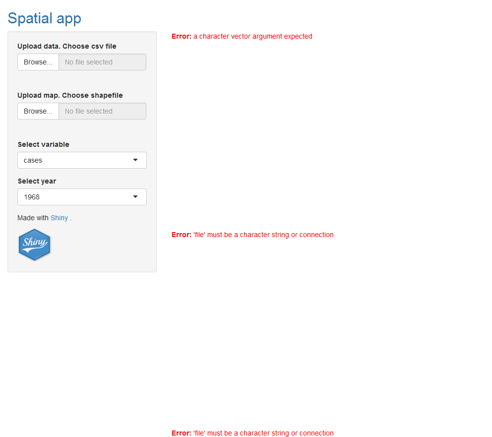
Figure 15.5: Snapshot of the Shiny app after adding inputs to upload the data and the map. The Shiny app renders error letters until the files are uploaded.
Requiring input files to be available using req()
First, inside the reactive expressions that read the files, we include req(input$inputId) to require input$inputId to be available before showing the outputs. req() evaluates its arguments 1 at a time and if these are missing the execution of the reactive expression stops. In this manner, the value returned by the reactive expression will not be updated, and outputs that employ the value returned by the reactive expression will not be reexecuted. Details on how to use req() are in the RStudio website.
We add req(input$filedata) at the beginning of the reactive expression that reads the data. If the data has non been uploaded yet, input$filedata is equal to "". This stops the execution of the reactive expression, so data() is not updated, and the output depending on data() is not executed.
# in ui. Outset line in the reactive() that reads the information req ( input $ filedata ) Similarly, we add req(input$filemap) at the beginning of the reactive expression that reads the map. If the map has not been uploaded nevertheless, input$filemap is missing, the execution of the reactive expression stops, map() is not updated, and the output depending on map() is not executed.
# in ui. First line in the reactive() that reads the map req ( input $ filemap ) Checking information are uploaded before creating the map
Before constructing the leaflet map, the data has to exist added to the shapefile. To do this, nosotros need to make sure that both the data and the map are uploaded. We can do this by writing at the start of renderLeaflet() the following code.
When either data() or map() are updated, the instructions of renderLeaflet() are executed. Then, at the beginning of renderLeaflet() it is checked whether either information() or map() are Nothing. If this is TRUE, the execution stops returning Nil. This avoids the fault that we would get when trying to add together the data to the map when either of these two elements is Zero.
Conclusion
In this affiliate, we accept shown how to create a Shiny app to upload and visualize spatio-temporal information. We accept shown how to upload a shapefile with a map and a CSV file with data, how to create interactive visualizations including a table with DT, a map with leaflet and a fourth dimension plot with dygraphs, and how to add reactivity that enables the user to evidence specific information. The complete lawmaking of the Shiny app is given beneath, and a snapshot of the Shiny app created is shown in Figure xv.1. Nosotros tin can improve the appearance and functionality of the Shiny app by modifying the layout and adding other inputs and outputs. The website http://shiny.rstudio.com/ contains multiple resources that can be used to improve the Shiny app.
library ( shiny ) library ( rgdal ) library ( DT ) library ( dygraphs ) library ( xts ) library ( leaflet ) # ui object ui <- fluidPage ( titlePanel ( p ( "Spatial app", style = "colour:#3474A7" ) ), sidebarLayout ( sidebarPanel ( fileInput ( inputId = "filedata", label = "Upload data. Choose csv file", accept = c ( ".csv" ) ), fileInput ( inputId = "filemap", label = "Upload map. Choose shapefile", multiple = TRUE, have = c ( ".shp", ".dbf", ".sbn", ".sbx", ".shx", ".prj" ) ), selectInput ( inputId = "variableselected", characterization = "Select variable", choices = c ( "cases", "population" ) ), selectInput ( inputId = "yearselected", label = "Select year", choices = 1968 : 1988 ), p ( "Fabricated with", a ( "Shiny", href = "http://shiny.rstudio.com" ), "." ), img ( src = "imageShiny.png", width = "70px", elevation = "70px" ) ), mainPanel ( leafletOutput (outputId = "map" ), dygraphOutput (outputId = "timetrend" ), DTOutput (outputId = "table" ) ) ) ) # server() server <- office ( input, output ) { data <- reactive ( { req ( input $ filedata ) read.csv ( input $ filedata $ datapath ) } ) map <- reactive ( { req ( input $ filemap ) # shpdf is a data.frame with the name, size, blazon and # datapath of the uploaded files shpdf <- input $ filemap # The files are uploaded with names # 0.dbf, one.prj, 2.shp, 3.xml, 4.shx # (path/names are in cavalcade datapath) # We need to rename the files with the actual names: # fe_2007_39_county.dbf, etc. # (these are in cavalcade name) # Proper noun of the temporary directory where files are uploaded tempdirname <- dirname ( shpdf $ datapath [ 1 ] ) # Rename files for ( i in 1 : nrow ( shpdf ) ) { file.rename ( shpdf $ datapath [ i ], paste0 ( tempdirname, "/", shpdf $ name [ i ] ) ) } # Now we read the shapefile with readOGR() of rgdal package # passing the name of the file with .shp extension. # Nosotros use the function grep() to search the pattern "*.shp$" # within each element of the graphic symbol vector shpdf$name. # grep(pattern="*.shp$", shpdf$name) # ($ at the end denote files that finish with .shp, # not only that incorporate .shp) map <- readOGR ( paste ( tempdirname, shpdf $ proper noun [ grep (blueprint = "*.shp$", shpdf $ name ) ], sep = "/" ) ) map } ) output $ tabular array <- renderDT ( information ( ) ) output $ timetrend <- renderDygraph ( { data <- information ( ) dataxts <- NULL counties <- unique ( data $ canton ) for ( fifty in 1 : length ( counties ) ) { datacounty <- information [ data $ county == counties [ l ], ] dd <- xts ( datacounty [, input $ variableselected ], as.Date ( paste0 ( datacounty $ year, "-01-01" ) ) ) dataxts <- cbind ( dataxts, dd ) } colnames ( dataxts ) <- counties dygraph ( dataxts ) %>% dyHighlight (highlightSeriesBackgroundAlpha = 0.2 ) -> d1 d1 $ x $ css <- " .dygraph-fable > span {brandish:none;} .dygraph-legend > span.highlight { brandish: inline; } " d1 } ) output $ map <- renderLeaflet ( { if ( is.null ( data ( ) ) | is.null ( map ( ) ) ) { return ( NULL ) } map <- map ( ) information <- data ( ) # Add information to map datafiltered <- data [ which ( data $ twelvemonth == input $ yearselected ), ] ordercounties <- friction match ( map @ data $ Proper noun, datafiltered $ county ) map @ data <- datafiltered [ ordercounties, ] # Create variableplot map $ variableplot <- as.numeric ( map @ data [, input $ variableselected ] ) # Create leaflet pal <- colorBin ( "YlOrRd", domain = map $ variableplot, bins = 7 ) labels <- sprintf ( "%s: %g", map $ canton, map $ variableplot ) %>% lapply ( htmltools :: HTML ) 50 <- leaflet ( map ) %>% addTiles ( ) %>% addPolygons ( fillColor = ~ pal ( variableplot ), color = "white", dashArray = "iii", fillOpacity = 0.vii, label = labels ) %>% leaflet :: addLegend ( pal = pal, values = ~ variableplot, opacity = 0.7, title = NULL ) } ) } # shinyApp() shinyApp (ui = ui, server = server ) Source: https://www.paulamoraga.com/book-geospatial/sec-shinyexample.html
0 Response to "How to Upload Text File and Display It in Shiny"
Enviar um comentário